最適化の解空間の輪郭を描く

等高線図は、最適化問題の解空間を示すときに特に便利です。axes.Axes.contour目的関数のトポグラフィを表すために使用できるだけでなく、制約関数の境界曲線を生成するためにも使用できます。で制約線を描画し TickedStrokeて、制約境界の有効な側と無効な側を区別できます。

axes.Axes.contour等高線の左側に大きな値を持つ曲線を生成します。角度パラメータはゼロ前方で測定され、左に向かって値が増加します。したがって、 を使用 TickedStrokeして典型的な最適化問題の制約を説明する場合、角度は 0 ～ 180 度に設定する必要があります。

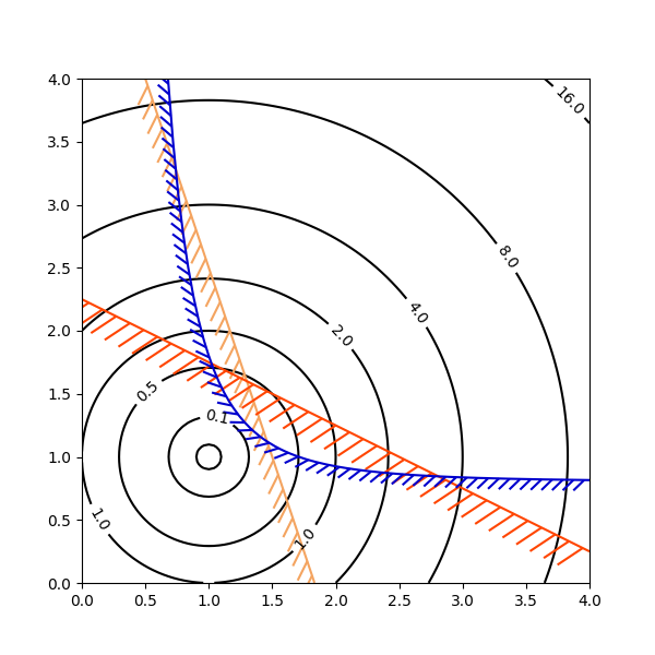
import numpy as np
import matplotlib.pyplot as plt
from matplotlib import patheffects

fig, ax = plt.subplots(figsize=(6, 6))

nx = 101
ny = 105

# Set up survey vectors
xvec = np.linspace(0.001, 4.0, nx)
yvec = np.linspace(0.001, 4.0, ny)

# Set up survey matrices.  Design disk loading and gear ratio.
x1, x2 = np.meshgrid(xvec, yvec)

# Evaluate some stuff to plot
obj = x1**2 + x2**2 - 2*x1 - 2*x2 + 2
g1 = -(3*x1 + x2 - 5.5)
g2 = -(x1 + 2*x2 - 4.5)
g3 = 0.8 + x1**-3 - x2

cntr = ax.contour(x1, x2, obj, [0.01, 0.1, 0.5, 1, 2, 4, 8, 16],
                  colors='black')
ax.clabel(cntr, fmt="%2.1f", use_clabeltext=True)

cg1 = ax.contour(x1, x2, g1, [0], colors='sandybrown')
plt.setp(cg1.collections,
         path_effects=[patheffects.withTickedStroke(angle=135)])

cg2 = ax.contour(x1, x2, g2, [0], colors='orangered')
plt.setp(cg2.collections,
         path_effects=[patheffects.withTickedStroke(angle=60, length=2)])

cg3 = ax.contour(x1, x2, g3, [0], colors='mediumblue')
plt.setp(cg3.collections,
         path_effects=[patheffects.withTickedStroke(spacing=7)])

ax.set_xlim(0, 4)
ax.set_ylim(0, 4)

plt.show()