pcolormesh #

axes.Axes.pcolormesh2D 画像スタイルのプロットを生成できます。同様のよりも高速であることに注意してくださいpcolor。

import matplotlib.pyplot as plt
from matplotlib.colors import BoundaryNorm
from matplotlib.ticker import MaxNLocator
import numpy as np

基本的なpcolormesh #

通常、四角形のエッジと四角形の値を定義することにより、pcolormesh を指定します。ここで、xとyはそれぞれ、それぞれの次元で Z よりも 1 つの余分な要素を持っていることに注意してください。

np.random.seed(19680801)
Z = np.random.rand(6, 10)
x = np.arange(-0.5, 10, 1)  # len = 11
y = np.arange(4.5, 11, 1)  # len = 7

fig, ax = plt.subplots()
ax.pcolormesh(x, y, Z)

<matplotlib.collections.QuadMesh object at 0x7f2d00aaeef0>

非直線的な pcolormesh #

XとYの行列を指定して、非直線の四辺形を指定することもできることに注意してください。

x = np.arange(-0.5, 10, 1)  # len = 11
y = np.arange(4.5, 11, 1)  # len = 7
X, Y = np.meshgrid(x, y)
X = X + 0.2 * Y  # tilt the coordinates.
Y = Y + 0.3 * X

fig, ax = plt.subplots()
ax.pcolormesh(X, Y, Z)

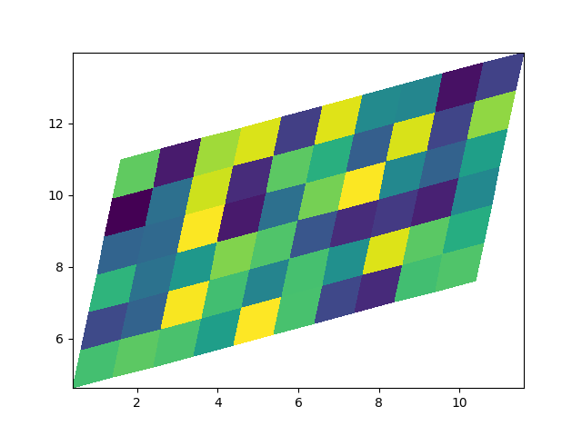
<matplotlib.collections.QuadMesh object at 0x7f2d00c610f0>

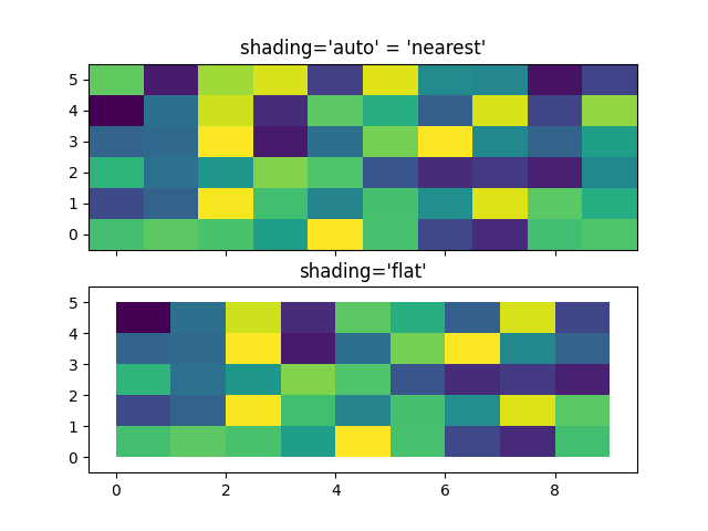
中心座標#

多くの場合、ユーザーはXとYをZと同じサイズでに渡したいと考えていaxes.Axes.pcolormeshます。shading='auto'これは、が渡された場合にも許可されます (デフォルトはrcParams["pcolor.shading"](default: 'auto') によって設定されます)。Matplotlib 3.3 より前では、 Zshading='flat'の最後の列と行が削除されます。これは後方互換性のために引き続き許可されていますが、DeprecationWarning が発生します。これが本当に必要な場合は、Z の最後の行と列を手動で削除するだけです。

x = np.arange(10)  # len = 10
y = np.arange(6)  # len = 6
X, Y = np.meshgrid(x, y)

fig, axs = plt.subplots(2, 1, sharex=True, sharey=True)
axs[0].pcolormesh(X, Y, Z, vmin=np.min(Z), vmax=np.max(Z), shading='auto')
axs[0].set_title("shading='auto' = 'nearest'")
axs[1].pcolormesh(X, Y, Z[:-1, :-1], vmin=np.min(Z), vmax=np.max(Z),
                  shading='flat')
axs[1].set_title("shading='flat'")

Text(0.5, 1.0, "shading='flat'")

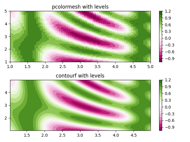
規範を使用してレベルを作成する#

Normalization と Colormap インスタンスを組み合わせてで「レベル」を描画しaxes.Axes.pcolor、contour/contourf の level キーワード引数と同様の方法でプロットを入力する方法を示しますaxes.Axes.pcolormesh 。axes.Axes.imshow

# make these smaller to increase the resolution
dx, dy = 0.05, 0.05

# generate 2 2d grids for the x & y bounds
y, x = np.mgrid[slice(1, 5 + dy, dy),
                slice(1, 5 + dx, dx)]

z = np.sin(x)**10 + np.cos(10 + y*x) * np.cos(x)

# x and y are bounds, so z should be the value *inside* those bounds.
# Therefore, remove the last value from the z array.
z = z[:-1, :-1]
levels = MaxNLocator(nbins=15).tick_values(z.min(), z.max())


# pick the desired colormap, sensible levels, and define a normalization
# instance which takes data values and translates those into levels.
cmap = plt.colormaps['PiYG']
norm = BoundaryNorm(levels, ncolors=cmap.N, clip=True)

fig, (ax0, ax1) = plt.subplots(nrows=2)

im = ax0.pcolormesh(x, y, z, cmap=cmap, norm=norm)
fig.colorbar(im, ax=ax0)
ax0.set_title('pcolormesh with levels')


# contours are *point* based plots, so convert our bound into point
# centers
cf = ax1.contourf(x[:-1, :-1] + dx/2.,
                  y[:-1, :-1] + dy/2., z, levels=levels,
                  cmap=cmap)
fig.colorbar(cf, ax=ax1)
ax1.set_title('contourf with levels')

# adjust spacing between subplots so `ax1` title and `ax0` tick labels
# don't overlap
fig.tight_layout()

plt.show()

参考文献

この例では、次の関数、メソッド、クラス、およびモジュールの使用が示されています。

スクリプトの合計実行時間: ( 0 分 1.467 秒)

Sphinx-Gallery によって生成されたギャラリー