ノート
完全なサンプルコードをダウンロードするには、ここをクリックしてください
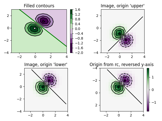
輪郭画像#
等高線、塗りつぶし等高線、および画像プロットの組み合わせをテストします。等高線のラベル付けについては、等高線のデモの例も参照してください。
このデモでは、輪郭を画像に正しく登録する方法と、両方を希望どおりに配置する方法を示すことに重点を置いています。特に、「origin」および「extent」キーワード引数を imshow および輪郭に使用することに注意してください。
import matplotlib.pyplot as plt
import numpy as np
from matplotlib import cm

# Default delta is large because that makes it fast, and it illustrates
# the correct registration between image and contours.
delta = 0.5

extent = (-3, 4, -4, 3)

x = np.arange(-3.0, 4.001, delta)
y = np.arange(-4.0, 3.001, delta)
X, Y = np.meshgrid(x, y)
Z1 = np.exp(-X**2 - Y**2)
Z2 = np.exp(-(X - 1)**2 - (Y - 1)**2)
Z = (Z1 - Z2) * 2

# Boost the upper limit to avoid truncation errors.
levels = np.arange(-2.0, 1.601, 0.4)

norm = cm.colors.Normalize(vmax=abs(Z).max(), vmin=-abs(Z).max())
cmap = cm.PRGn

fig, _axs = plt.subplots(nrows=2, ncols=2)
fig.subplots_adjust(hspace=0.3)
axs = _axs.flatten()

cset1 = axs[0].contourf(X, Y, Z, levels, norm=norm,
                        cmap=cmap.resampled(len(levels) - 1))
# It is not necessary, but for the colormap, we need only the
# number of levels minus 1.  To avoid discretization error, use
# either this number or a large number such as the default (256).

# If we want lines as well as filled regions, we need to call
# contour separately; don't try to change the edgecolor or edgewidth
# of the polygons in the collections returned by contourf.
# Use levels output from previous call to guarantee they are the same.

cset2 = axs[0].contour(X, Y, Z, cset1.levels, colors='k')

# We don't really need dashed contour lines to indicate negative
# regions, so let's turn them off.

for c in cset2.collections:
    c.set_linestyle('solid')

# It is easier here to make a separate call to contour than
# to set up an array of colors and linewidths.
# We are making a thick green line as a zero contour.
# Specify the zero level as a tuple with only 0 in it.

cset3 = axs[0].contour(X, Y, Z, (0,), colors='g', linewidths=2)
axs[0].set_title('Filled contours')
fig.colorbar(cset1, ax=axs[0])


axs[1].imshow(Z, extent=extent, cmap=cmap, norm=norm)
axs[1].contour(Z, levels, colors='k', origin='upper', extent=extent)
axs[1].set_title("Image, origin 'upper'")

axs[2].imshow(Z, origin='lower', extent=extent, cmap=cmap, norm=norm)
axs[2].contour(Z, levels, colors='k', origin='lower', extent=extent)
axs[2].set_title("Image, origin 'lower'")

# We will use the interpolation "nearest" here to show the actual
# image pixels.
# Note that the contour lines don't extend to the edge of the box.
# This is intentional. The Z values are defined at the center of each
# image pixel (each color block on the following subplot), so the
# domain that is contoured does not extend beyond these pixel centers.
im = axs[3].imshow(Z, interpolation='nearest', extent=extent,
                   cmap=cmap, norm=norm)
axs[3].contour(Z, levels, colors='k', origin='image', extent=extent)
ylim = axs[3].get_ylim()
axs[3].set_ylim(ylim[::-1])
axs[3].set_title("Origin from rc, reversed y-axis")
fig.colorbar(im, ax=axs[3])

fig.tight_layout()
plt.show()
参考文献
この例では、次の関数、メソッド、クラス、およびモジュールの使用が示されています。