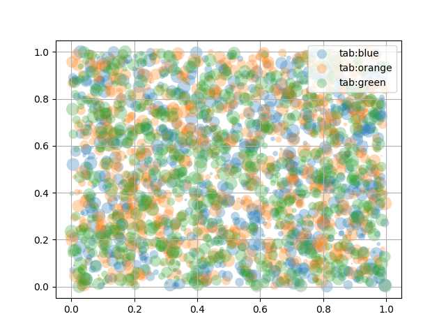
凡例付きの散布図#

scatter凡例付きの散布図を作成するには、ループを使用して項目ごとに1 つのプロットを作成し、凡例に表示して、label それに応じてを設定します。

alpha以下は、0 から 1 の間の値を指定してマーカーの透明度を調整する方法も示しています。

import numpy as np
import matplotlib.pyplot as plt

np.random.seed(19680801)


fig, ax = plt.subplots()
for color in ['tab:blue', 'tab:orange', 'tab:green']:
    n = 750
    x, y = np.random.rand(2, n)
    scale = 200.0 * np.random.rand(n)
    ax.scatter(x, y, c=color, s=scale, label=color,
               alpha=0.3, edgecolors='none')

ax.legend()
ax.grid(True)

plt.show()

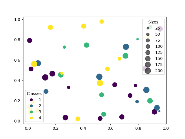
凡例の自動作成#

散布図の凡例を作成する別のオプションは、 PathCollection.legend_elementsメソッドを使用することです。表示する凡例エントリの有用な数を自動的に決定しようとし、ハンドルとラベルのタプルを返します。これらはへの呼び出しに渡すことができますlegend。

N = 45
x, y = np.random.rand(2, N)
c = np.random.randint(1, 5, size=N)
s = np.random.randint(10, 220, size=N)

fig, ax = plt.subplots()

scatter = ax.scatter(x, y, c=c, s=s)

# produce a legend with the unique colors from the scatter
legend1 = ax.legend(*scatter.legend_elements(),
                    loc="lower left", title="Classes")
ax.add_artist(legend1)

# produce a legend with a cross section of sizes from the scatter
handles, labels = scatter.legend_elements(prop="sizes", alpha=0.6)
legend2 = ax.legend(handles, labels, loc="upper right", title="Sizes")

plt.show()

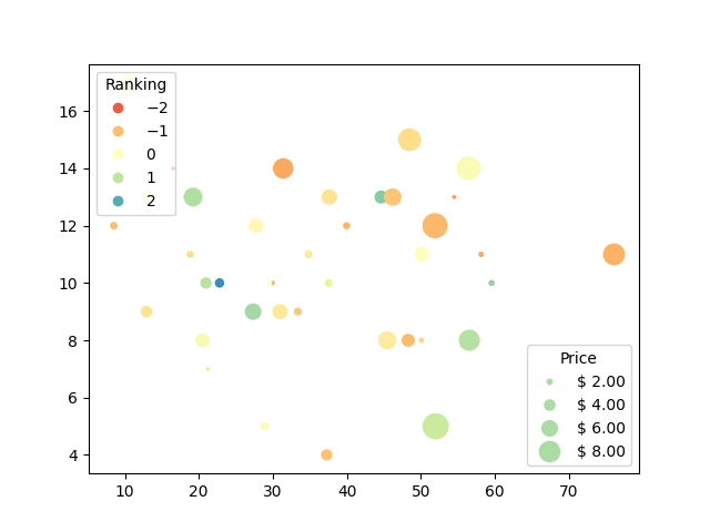
メソッドへの追加の引数をPathCollection.legend_elements使用して、作成する凡例エントリの数とそれらのラベル付け方法を操作できます。以下にその一部の使用方法を示します。

volume = np.random.rayleigh(27, size=40)
amount = np.random.poisson(10, size=40)
ranking = np.random.normal(size=40)
price = np.random.uniform(1, 10, size=40)

fig, ax = plt.subplots()

# Because the price is much too small when being provided as size for ``s``,
# we normalize it to some useful point sizes, s=0.3*(price*3)**2
scatter = ax.scatter(volume, amount, c=ranking, s=0.3*(price*3)**2,
                     vmin=-3, vmax=3, cmap="Spectral")

# Produce a legend for the ranking (colors). Even though there are 40 different
# rankings, we only want to show 5 of them in the legend.
legend1 = ax.legend(*scatter.legend_elements(num=5),
                    loc="upper left", title="Ranking")
ax.add_artist(legend1)

# Produce a legend for the price (sizes). Because we want to show the prices
# in dollars, we use the *func* argument to supply the inverse of the function
# used to calculate the sizes from above. The *fmt* ensures to show the price
# in dollars. Note how we target at 5 elements here, but obtain only 4 in the
# created legend due to the automatic round prices that are chosen for us.
kw = dict(prop="sizes", num=5, color=scatter.cmap(0.7), fmt="$ {x:.2f}",
          func=lambda s: np.sqrt(s/.3)/3)
legend2 = ax.legend(*scatter.legend_elements(**kw),
                    loc="lower right", title="Price")

plt.show()

参考文献

この例では、次の関数、メソッド、クラス、およびモジュールの使用が示されています。

スクリプトの合計実行時間: ( 0 分 1.840 秒)

Sphinx-Gallery によって生成されたギャラリー