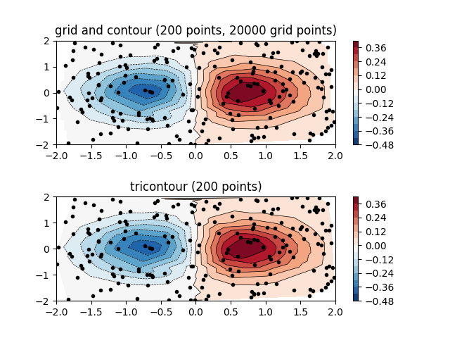
不規則な間隔のデータの等高線図#

規則的なグリッドで補間された不規則な間隔のデータのコンタープロットと、構造化されていない三角グリッドのトライコンタープロットの比較。

データが規則的なグリッド上に存在することが期待されるためcontour、contourf不規則な間隔のデータの等高線図をプロットするには、さまざまな方法が必要です。2 つのオプションは次のとおりです。

最初にデータを通常のグリッドに補間します。これは、オンボードの手段を使用してLinearTriInterpolator、または外部機能を使用して行うことができますscipy.interpolate.griddata。次に、補間されたデータを通常のでプロットしますcontour。
内部で三角測量を実行するtricontourorを直接使用します。tricontourf

この例では、両方のメソッドの動作を示しています。

import matplotlib.pyplot as plt
import matplotlib.tri as tri
import numpy as np

np.random.seed(19680801)
npts = 200
ngridx = 100
ngridy = 200
x = np.random.uniform(-2, 2, npts)
y = np.random.uniform(-2, 2, npts)
z = x * np.exp(-x**2 - y**2)

fig, (ax1, ax2) = plt.subplots(nrows=2)

# -----------------------
# Interpolation on a grid
# -----------------------
# A contour plot of irregularly spaced data coordinates
# via interpolation on a grid.

# Create grid values first.
xi = np.linspace(-2.1, 2.1, ngridx)
yi = np.linspace(-2.1, 2.1, ngridy)

# Linearly interpolate the data (x, y) on a grid defined by (xi, yi).
triang = tri.Triangulation(x, y)
interpolator = tri.LinearTriInterpolator(triang, z)
Xi, Yi = np.meshgrid(xi, yi)
zi = interpolator(Xi, Yi)

# Note that scipy.interpolate provides means to interpolate data on a grid
# as well. The following would be an alternative to the four lines above:
# from scipy.interpolate import griddata
# zi = griddata((x, y), z, (xi[None, :], yi[:, None]), method='linear')

ax1.contour(xi, yi, zi, levels=14, linewidths=0.5, colors='k')
cntr1 = ax1.contourf(xi, yi, zi, levels=14, cmap="RdBu_r")

fig.colorbar(cntr1, ax=ax1)
ax1.plot(x, y, 'ko', ms=3)
ax1.set(xlim=(-2, 2), ylim=(-2, 2))
ax1.set_title('grid and contour (%d points, %d grid points)' %
              (npts, ngridx * ngridy))

# ----------
# Tricontour
# ----------
# Directly supply the unordered, irregularly spaced coordinates
# to tricontour.

ax2.tricontour(x, y, z, levels=14, linewidths=0.5, colors='k')
cntr2 = ax2.tricontourf(x, y, z, levels=14, cmap="RdBu_r")

fig.colorbar(cntr2, ax=ax2)
ax2.plot(x, y, 'ko', ms=3)
ax2.set(xlim=(-2, 2), ylim=(-2, 2))
ax2.set_title('tricontour (%d points)' % npts)

plt.subplots_adjust(hspace=0.5)
plt.show()

グリッドとコンター (200 ポイント、20000 グリッドポイント)、tricontour (200 ポイント)

参考文献

この例では、次の関数、メソッド、クラス、およびモジュールの使用が示されています。

Sphinx-Gallery によって生成されたギャラリー