輪郭のデモ#

単純な等高線図、等高線用のカラーバーを使用したイメージ上の等高線、およびラベル付きの等高線を示します。

輪郭画像の例も参照してください。

import numpy as np
import matplotlib.cm as cm
import matplotlib.pyplot as plt


delta = 0.025
x = np.arange(-3.0, 3.0, delta)
y = np.arange(-2.0, 2.0, delta)
X, Y = np.meshgrid(x, y)
Z1 = np.exp(-X**2 - Y**2)
Z2 = np.exp(-(X - 1)**2 - (Y - 1)**2)
Z = (Z1 - Z2) * 2

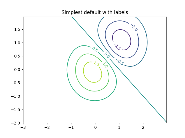
既定の色を使用してラベルを付けた単純な等高線図を作成します。clabel の inline 引数は、ラベルが等高線の線分の上に描画され、ラベルの下の線が削除されるかどうかを制御します。

fig, ax = plt.subplots()
CS = ax.contour(X, Y, Z)
ax.clabel(CS, inline=True, fontsize=10)
ax.set_title('Simplest default with labels')

Text(0.5, 1.0, 'Simplest default with labels')

位置のリストを (データ座標で) 提供することにより、等高線ラベルを手動で配置できます。インタラクティブな配置については、インタラクティブ関数を参照してください。

fig, ax = plt.subplots()
CS = ax.contour(X, Y, Z)
manual_locations = [
    (-1, -1.4), (-0.62, -0.7), (-2, 0.5), (1.7, 1.2), (2.0, 1.4), (2.4, 1.7)]
ax.clabel(CS, inline=True, fontsize=10, manual=manual_locations)
ax.set_title('labels at selected locations')

Text(0.5, 1.0, 'labels at selected locations')

すべての輪郭を強制的に同じ色にすることができます。

fig, ax = plt.subplots()
CS = ax.contour(X, Y, Z, 6, colors='k')  # Negative contours default to dashed.
ax.clabel(CS, fontsize=9, inline=True)
ax.set_title('Single color - negative contours dashed')

Text(0.5, 1.0, 'Single color - negative contours dashed')

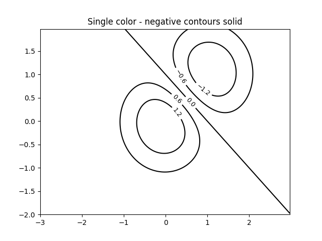
負の等高線を破線ではなく実線に設定できます。

plt.rcParams['contour.negative_linestyle'] = 'solid'
fig, ax = plt.subplots()
CS = ax.contour(X, Y, Z, 6, colors='k')  # Negative contours default to dashed.
ax.clabel(CS, fontsize=9, inline=True)
ax.set_title('Single color - negative contours solid')

Text(0.5, 1.0, 'Single color - negative contours solid')

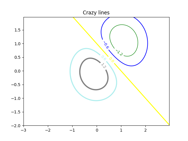
また、輪郭の色を手動で指定できます

fig, ax = plt.subplots()
CS = ax.contour(X, Y, Z, 6,
                linewidths=np.arange(.5, 4, .5),
                colors=('r', 'green', 'blue', (1, 1, 0), '#afeeee', '0.5'),
                )
ax.clabel(CS, fontsize=9, inline=True)
ax.set_title('Crazy lines')

Text(0.5, 1.0, 'Crazy lines')

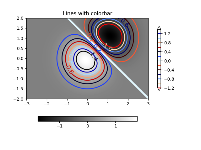
または、カラーマップを使用して色を指定できます。デフォルトのカラーマップが等高線に使用されます

fig, ax = plt.subplots()
im = ax.imshow(Z, interpolation='bilinear', origin='lower',
               cmap=cm.gray, extent=(-3, 3, -2, 2))
levels = np.arange(-1.2, 1.6, 0.2)
CS = ax.contour(Z, levels, origin='lower', cmap='flag', extend='both',
                linewidths=2, extent=(-3, 3, -2, 2))

# Thicken the zero contour.
CS.collections[6].set_linewidth(4)

ax.clabel(CS, levels[1::2],  # label every second level
          inline=True, fmt='%1.1f', fontsize=14)

# make a colorbar for the contour lines
CB = fig.colorbar(CS, shrink=0.8)

ax.set_title('Lines with colorbar')

# We can still add a colorbar for the image, too.
CBI = fig.colorbar(im, orientation='horizontal', shrink=0.8)

# This makes the original colorbar look a bit out of place,
# so let's improve its position.

l, b, w, h = ax.get_position().bounds
ll, bb, ww, hh = CB.ax.get_position().bounds
CB.ax.set_position([ll, b + 0.1*h, ww, h*0.8])

plt.show()

参考文献

この例では、次の関数、メソッド、クラス、およびモジュールの使用が示されています。

スクリプトの合計実行時間: ( 0 分 2.685 秒)

Sphinx-Gallery によって生成されたギャラリー