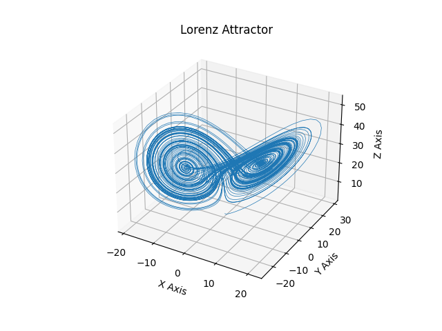
ローレンツ アトラクタ

これはエドワード・ローレンツの 1963 年の「決定論的非周期的フロー」を mplot3d を使用して 3 次元空間にプロットした例です。

ノート

これは単純な非線形 ODE であるため、SciPy の ODE ソルバーを使用するとより簡単に実行できますが、このアプローチは NumPy のみに依存しています。

import numpy as np
import matplotlib.pyplot as plt


def lorenz(xyz, *, s=10, r=28, b=2.667):
    """
    Parameters
    ----------
    xyz : array-like, shape (3,)
       Point of interest in three dimensional space.
    s, r, b : float
       Parameters defining the Lorenz attractor.

    Returns
    -------
    xyz_dot : array, shape (3,)
       Values of the Lorenz attractor's partial derivatives at *xyz*.
    """
    x, y, z = xyz
    x_dot = s*(y - x)
    y_dot = r*x - y - x*z
    z_dot = x*y - b*z
    return np.array([x_dot, y_dot, z_dot])


dt = 0.01
num_steps = 10000

xyzs = np.empty((num_steps + 1, 3))  # Need one more for the initial values
xyzs[0] = (0., 1., 1.05)  # Set initial values
# Step through "time", calculating the partial derivatives at the current point
# and using them to estimate the next point
for i in range(num_steps):
    xyzs[i + 1] = xyzs[i] + lorenz(xyzs[i]) * dt

# Plot
ax = plt.figure().add_subplot(projection='3d')

ax.plot(*xyzs.T, lw=0.5)
ax.set_xlabel("X Axis")
ax.set_ylabel("Y Axis")
ax.set_zlabel("Z Axis")
ax.set_title("Lorenz Attractor")

plt.show()