ノート
完全なサンプルコードをダウンロードするには、ここをクリックしてください
色のリストからカラーマップを作成する#
カラーマップの作成と操作の詳細については、 Creating Colormaps in Matplotlibを参照してください。
メソッドを使用して、色のリストからカラーマップを作成できますLinearSegmentedColormap.from_list。0 から 1 までの色の混合を定義する RGB タプルのリストを渡す必要があります。
カスタムカラーマップの作成#
カラーマップのカスタム マッピングを作成することもできます。これは、RGB チャネルが cmap の一方の端から他方の端にどのように変化するかを指定するディクショナリを作成することによって実現されます。
例: 赤を下半分で 0 から 1 に増やし、緑を中半分で同じように増やし、青を上半分で増やしたいとします。次に、次を使用します。
cdict = {
    'red': (
        (0.0,  0.0, 0.0),
        (0.5,  1.0, 1.0),
        (1.0,  1.0, 1.0),
    ),
    'green': (
        (0.0,  0.0, 0.0),
        (0.25, 0.0, 0.0),
        (0.75, 1.0, 1.0),
        (1.0,  1.0, 1.0),
    ),
    'blue': (
        (0.0,  0.0, 0.0),
        (0.5,  0.0, 0.0),
        (1.0,  1.0, 1.0),
    )
}
この例のように、r、g、および b コンポーネントに不連続性がない場合は、非常に単純です。上記の各タプルの 2 番目と 3 番目の要素は同じで、" y" と呼びます。最初の要素 (" x") は、0 から 1 の全範囲にわたる補間間隔を定義し、その範囲全体にまたがる必要があります。つまり、 の値はx0 から 1 の範囲を一連のセグメントに分割しy、各セグメントのエンドポイント カラー値を提供します。
次に、緑について考えてみましょうcdict['green']。
0 <=
x<= 0.25、yゼロです。緑なし。0.25 <
x<= 0.75、0yから 1 まで直線的に変化します。0.75 <
x<= 1、1 のyまま、完全な緑色。
不連続性がある場合は、もう少し複雑です。cdict特定の色のエントリの各行の 3 つの要素に としてラベルを付けます。次に、 と の間の値について、色の値がとの間で補間されます。(x, y0,
y1)xx[i]x[i+1]y1[i]y0[i+1]
クックブックの例に戻ります。
cdict = {
    'red': (
        (0.0,  0.0, 0.0),
        (0.5,  1.0, 0.7),
        (1.0,  1.0, 1.0),
    ),
    'green': (
        (0.0,  0.0, 0.0),
        (0.5,  1.0, 0.0),
        (1.0,  1.0, 1.0),
    ),
    'blue': (
        (0.0,  0.0, 0.0),
        (0.5,  0.0, 0.0),
        (1.0,  1.0, 1.0),
    )
}
そして見てくださいcdict['red'][1]。なぜなら、
0 から 0.5 まで、赤は 0 から 1 まで増加しますが、その後、赤が 0.5 から 1 まで増加すると、赤は 0.7 から 1 まで増加します。緑は 0 から 1 まで増加します。 0.5 にジャンプし、0 にジャンプして戻り、
0.5 から 1 になると 1 に戻ります。y0 != y1xxxx
x上記は、 から までの範囲x[i]でx[i+1]、補間が と の間でy1[i]あることを示す試みy0[i+1]です。したがって、y0[0]および
y1[-1]使用されることはありません。
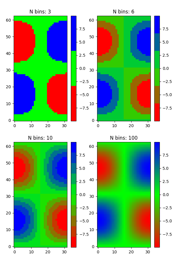
リストからのカラーマップ#
colors = [(1, 0, 0), (0, 1, 0), (0, 0, 1)]  # R -> G -> B
n_bins = [3, 6, 10, 100]  # Discretizes the interpolation into bins
cmap_name = 'my_list'
fig, axs = plt.subplots(2, 2, figsize=(6, 9))
fig.subplots_adjust(left=0.02, bottom=0.06, right=0.95, top=0.94, wspace=0.05)
for n_bin, ax in zip(n_bins, axs.flat):
    # Create the colormap
    cmap = LinearSegmentedColormap.from_list(cmap_name, colors, N=n_bin)
    # Fewer bins will result in "coarser" colomap interpolation
    im = ax.imshow(Z, origin='lower', cmap=cmap)
    ax.set_title("N bins: %s" % n_bin)
    fig.colorbar(im, ax=ax)
カスタムカラーマップ#
cdict1 = {
    'red': (
        (0.0, 0.0, 0.0),
        (0.5, 0.0, 0.1),
        (1.0, 1.0, 1.0),
    ),
    'green': (
        (0.0, 0.0, 0.0),
        (1.0, 0.0, 0.0),
    ),
    'blue': (
        (0.0, 0.0, 1.0),
        (0.5, 0.1, 0.0),
        (1.0, 0.0, 0.0),
    )
}

cdict2 = {
    'red': (
        (0.0, 0.0, 0.0),
        (0.5, 0.0, 1.0),
        (1.0, 0.1, 1.0),
    ),
    'green': (
        (0.0, 0.0, 0.0),
        (1.0, 0.0, 0.0),
    ),
    'blue': (
        (0.0, 0.0, 0.1),
        (0.5, 1.0, 0.0),
        (1.0, 0.0, 0.0),
    )
}

cdict3 = {
    'red': (
        (0.0, 0.0, 0.0),
        (0.25, 0.0, 0.0),
        (0.5, 0.8, 1.0),
        (0.75, 1.0, 1.0),
        (1.0, 0.4, 1.0),
    ),
    'green': (
        (0.0, 0.0, 0.0),
        (0.25, 0.0, 0.0),
        (0.5, 0.9, 0.9),
        (0.75, 0.0, 0.0),
        (1.0, 0.0, 0.0),
    ),
    'blue': (
        (0.0, 0.0, 0.4),
        (0.25, 1.0, 1.0),
        (0.5, 1.0, 0.8),
        (0.75, 0.0, 0.0),
        (1.0, 0.0, 0.0),
    )
}

# Make a modified version of cdict3 with some transparency
# in the middle of the range.
cdict4 = {
    **cdict3,
    'alpha': (
        (0.0, 1.0, 1.0),
        # (0.25, 1.0, 1.0),
        (0.5, 0.3, 0.3),
        # (0.75, 1.0, 1.0),
        (1.0, 1.0, 1.0),
    ),
}
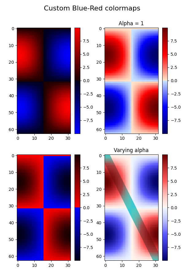
この例を使用して、カスタム カラーマップを処理する 2 つの方法を説明します。まず、最も直接的で明示的なもの:
blue_red1 = LinearSegmentedColormap('BlueRed1', cdict1)
次に、マップを明示的に作成して登録します。最初の方法と同様に、この方法は LinearSegmentedColormap だけでなく、あらゆる種類の Colormap で機能します。
mpl.colormaps.register(LinearSegmentedColormap('BlueRed2', cdict2))
mpl.colormaps.register(LinearSegmentedColormap('BlueRed3', cdict3))
mpl.colormaps.register(LinearSegmentedColormap('BlueRedAlpha', cdict4))
4 つのサブプロットを使用して図を作成します。
fig, axs = plt.subplots(2, 2, figsize=(6, 9))
fig.subplots_adjust(left=0.02, bottom=0.06, right=0.95, top=0.94, wspace=0.05)

im1 = axs[0, 0].imshow(Z, cmap=blue_red1)
fig.colorbar(im1, ax=axs[0, 0])

im2 = axs[1, 0].imshow(Z, cmap='BlueRed2')
fig.colorbar(im2, ax=axs[1, 0])

# Now we will set the third cmap as the default.  One would
# not normally do this in the middle of a script like this;
# it is done here just to illustrate the method.

plt.rcParams['image.cmap'] = 'BlueRed3'

im3 = axs[0, 1].imshow(Z)
fig.colorbar(im3, ax=axs[0, 1])
axs[0, 1].set_title("Alpha = 1")

# Or as yet another variation, we can replace the rcParams
# specification *before* the imshow with the following *after*
# imshow.
# This sets the new default *and* sets the colormap of the last
# image-like item plotted via pyplot, if any.
#

# Draw a line with low zorder so it will be behind the image.
axs[1, 1].plot([0, 10 * np.pi], [0, 20 * np.pi], color='c', lw=20, zorder=-1)

im4 = axs[1, 1].imshow(Z)
fig.colorbar(im4, ax=axs[1, 1])

# Here it is: changing the colormap for the current image and its
# colorbar after they have been plotted.
im4.set_cmap('BlueRedAlpha')
axs[1, 1].set_title("Varying alpha")

fig.suptitle('Custom Blue-Red colormaps', fontsize=16)
fig.subplots_adjust(top=0.9)

plt.show()
参考文献
この例では、次の関数、メソッド、クラス、およびモジュールの使用が示されています。
スクリプトの合計実行時間: ( 0 分 1.919 秒)