ノート

完全なサンプルコードをダウンロードするには、ここをクリックしてください

制約付きレイアウトガイド#

制約付きレイアウトを使用して、図内にプロットをきれいに収める方法。

Constrained_layoutは、凡例やカラーバーなどのサブプロットと装飾を自動的に調整して、ユーザーが要求した論理レイアウトを可能な限り維持しながら Figure ウィンドウに収まるようにします。

Constrained_layoutはtight_layoutに似ていますが、制約ソルバーを使用して、軸が収まるサイズを決定します。

通常、 constrained_layoutは、軸を Figure に追加する前にアクティブにする必要があります。その方法は 2 つあります。

subplots()またはにそれぞれの引数を使用しますfigure()。例:
```
plt.subplots(layout="constrained")
```
次のように、 rcParamsを介してアクティブ化します。
```
plt.rcParams['figure.constrained_layout.use'] = True
```

これらについては、以降のセクションで詳しく説明します。

簡単な例#

Matplotlib では、軸 (サブプロットを含む) の位置は正規化された Figure 座標で指定されます。軸ラベルまたはタイトル (場合によっては目盛りラベル) が Figure 領域の外に出て、切り取られることがあります。

import matplotlib.pyplot as plt
import matplotlib.colors as mcolors
import matplotlib.gridspec as gridspec
import numpy as np

plt.rcParams['savefig.facecolor'] = "0.8"
plt.rcParams['figure.figsize'] = 4.5, 4.
plt.rcParams['figure.max_open_warning'] = 50


def example_plot(ax, fontsize=12, hide_labels=False):
    ax.plot([1, 2])

    ax.locator_params(nbins=3)
    if hide_labels:
        ax.set_xticklabels([])
        ax.set_yticklabels([])
    else:
        ax.set_xlabel('x-label', fontsize=fontsize)
        ax.set_ylabel('y-label', fontsize=fontsize)
        ax.set_title('Title', fontsize=fontsize)

fig, ax = plt.subplots(layout=None)
example_plot(ax, fontsize=24)

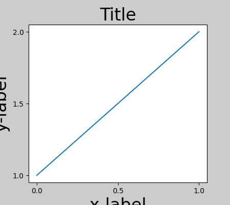
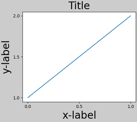
これを防ぐには、軸の位置を調整する必要があります。サブプロットの場合、これはを使用してサブプロットパラメータを調整することで手動で行うことができますFigure.subplots_adjust。ただし、 #layout="constrained"キーワード引数で図を指定すると、 # が自動的に調整されます。

fig, ax = plt.subplots(layout="constrained")
example_plot(ax, fontsize=24)

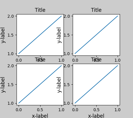
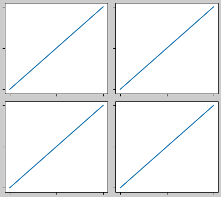
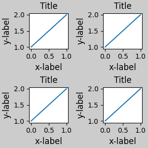
複数のサブプロットがある場合、異なる軸のラベルが互いに重なっていることがよくあります。

fig, axs = plt.subplots(2, 2, layout=None)
for ax in axs.flat:
    example_plot(ax)

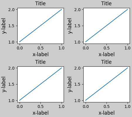
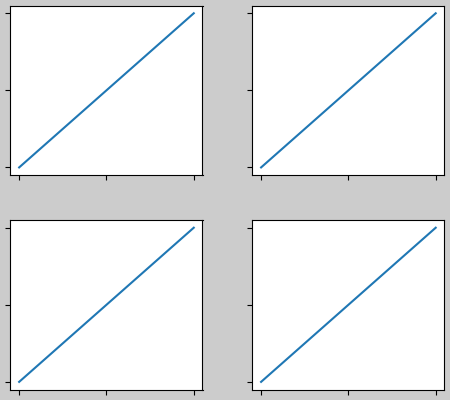
layout="constrained"の呼び出しで指定するplt.subplots と、レイアウトが適切に制約されます。

fig, axs = plt.subplots(2, 2, layout="constrained")
for ax in axs.flat:
    example_plot(ax)

カラーバー#

でカラーバーを作成する場合は、そのためのスペースを確保Figure.colorbarする必要があります。constrained_layoutこれを自動的に行います。use_gridspec=Trueこのオプションは経由でレイアウトを改善するために作成されているため、指定しても無視されることに注意してくださいtight_layout。

ノート

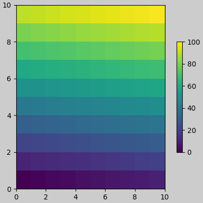
pcolormeshキーワード引数 ( ) にはpc_kwargs辞書を使用します。ScalarMappable以下では、それぞれが;を含むいくつかの軸に 1 つのカラーバーを割り当てます。ノルムとカラーマップを指定すると、カラーバーがすべての軸に対して正確になります。

arr = np.arange(100).reshape((10, 10))
norm = mcolors.Normalize(vmin=0., vmax=100.)
# see note above: this makes all pcolormesh calls consistent:
pc_kwargs = {'rasterized': True, 'cmap': 'viridis', 'norm': norm}
fig, ax = plt.subplots(figsize=(4, 4), layout="constrained")
im = ax.pcolormesh(arr, **pc_kwargs)
fig.colorbar(im, ax=ax, shrink=0.6)

<matplotlib.colorbar.Colorbar object at 0x7f2cfafb53c0>

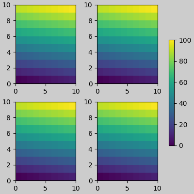
axの引数に軸 (または他の反復可能なコンテナー) のリストを指定するとcolorbar、constrained_layout は指定された軸からスペースを取ります。

fig, axs = plt.subplots(2, 2, figsize=(4, 4), layout="constrained")
for ax in axs.flat:
    im = ax.pcolormesh(arr, **pc_kwargs)
fig.colorbar(im, ax=axs, shrink=0.6)

<matplotlib.colorbar.Colorbar object at 0x7f2cfb6eed70>

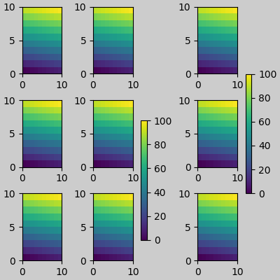
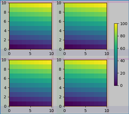
軸のグリッド内から軸のリストを指定すると、カラーバーは適切にスペースを奪い、ギャップを残しますが、すべてのサブプロットは同じサイズのままです。

fig, axs = plt.subplots(3, 3, figsize=(4, 4), layout="constrained")
for ax in axs.flat:
    im = ax.pcolormesh(arr, **pc_kwargs)
fig.colorbar(im, ax=axs[1:, ][:, 1], shrink=0.8)
fig.colorbar(im, ax=axs[:, -1], shrink=0.6)

<matplotlib.colorbar.Colorbar object at 0x7f2cdd1a3340>

副題番号

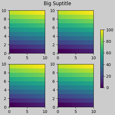
constrained_layoutのためのスペースを作ることもできますsuptitle。

fig, axs = plt.subplots(2, 2, figsize=(4, 4), layout="constrained")
for ax in axs.flat:
    im = ax.pcolormesh(arr, **pc_kwargs)
fig.colorbar(im, ax=axs, shrink=0.6)
fig.suptitle('Big Suptitle')

Text(0.5, 0.9895825, 'Big Suptitle')

伝説#

凡例は、親軸の外側に配置できます。Constrained-layout は、でこれを処理するように設計されていAxes.legend()ます。ただし、constrained-layout は(まだ)経由で作成された凡例を処理しません。Figure.legend()

fig, ax = plt.subplots(layout="constrained")
ax.plot(np.arange(10), label='This is a plot')
ax.legend(loc='center left', bbox_to_anchor=(0.8, 0.5))

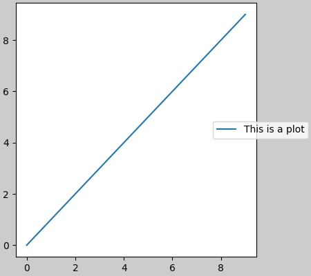
<matplotlib.legend.Legend object at 0x7f2cfb266d70>

ただし、これはサブプロットレイアウトからスペースを奪います。

fig, axs = plt.subplots(1, 2, figsize=(4, 2), layout="constrained")
axs[0].plot(np.arange(10))
axs[1].plot(np.arange(10), label='This is a plot')
axs[1].legend(loc='center left', bbox_to_anchor=(0.8, 0.5))

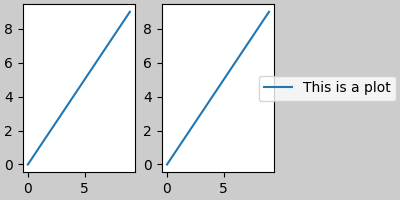
<matplotlib.legend.Legend object at 0x7f2cf99852a0>

レジェンドや他のアーティストがサブプロットのレイアウトからスペースを盗まないleg.set_in_layout(False)ようにするために、 . もちろん、これは凡例がトリミングされることを意味する可能性がありますが、後でプロットがで呼び出される場合に役立ちます。ただし、保存したファイルを機能させるには、凡例のステータスを再度切り替える必要があることに注意してください。また、constrained_layout で軸のサイズを調整して印刷する場合は、手動で描画をトリガーする必要があります。fig.savefig('outname.png', bbox_inches='tight')get_in_layout

fig, axs = plt.subplots(1, 2, figsize=(4, 2), layout="constrained")

axs[0].plot(np.arange(10))
axs[1].plot(np.arange(10), label='This is a plot')
leg = axs[1].legend(loc='center left', bbox_to_anchor=(0.8, 0.5))
leg.set_in_layout(False)
# trigger a draw so that constrained_layout is executed once
# before we turn it off when printing....
fig.canvas.draw()
# we want the legend included in the bbox_inches='tight' calcs.
leg.set_in_layout(True)
# we don't want the layout to change at this point.
fig.set_layout_engine(None)
try:
    fig.savefig('../../doc/_static/constrained_layout_1b.png',
                bbox_inches='tight', dpi=100)
except FileNotFoundError:
    # this allows the script to keep going if run interactively and
    # the directory above doesn't exist
    pass

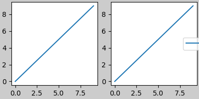
保存されたファイルは次のようになります。

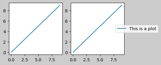
このぎこちなさを回避するより良い方法は、単純にが提供する凡例メソッドを使用することFigure.legendです。

fig, axs = plt.subplots(1, 2, figsize=(4, 2), layout="constrained")
axs[0].plot(np.arange(10))
lines = axs[1].plot(np.arange(10), label='This is a plot')
labels = [l.get_label() for l in lines]
leg = fig.legend(lines, labels, loc='center left',
                 bbox_to_anchor=(0.8, 0.5), bbox_transform=axs[1].transAxes)
try:
    fig.savefig('../../doc/_static/constrained_layout_2b.png',
                bbox_inches='tight', dpi=100)
except FileNotFoundError:
    # this allows the script to keep going if run interactively and
    # the directory above doesn't exist
    pass

保存されたファイルは次のようになります。

パディングとスペース#

軸間のパディングは、 w_pad と wspace によって水平方向に制御され、h_padとhspaceによって垂直方向に制御されます。これらはで編集できます。w/h_padは、軸の周囲の最小スペース (インチ単位) です。set

fig, axs = plt.subplots(2, 2, layout="constrained")
for ax in axs.flat:
    example_plot(ax, hide_labels=True)
fig.get_layout_engine().set(w_pad=4 / 72, h_pad=4 / 72, hspace=0,
                            wspace=0)

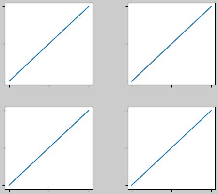
サブプロット間の間隔は、 wspaceおよびhspaceによってさらに設定されます。これらは、サブプロットグループ全体のサイズの一部として指定されます。これらの値がw_padまたはh_padより小さい場合、代わりに固定パッドが使用されます。以下では、エッジのスペースが上記から変化しないことに注意してください。ただし、サブプロット間のスペースは変化します。

fig, axs = plt.subplots(2, 2, layout="constrained")
for ax in axs.flat:
    example_plot(ax, hide_labels=True)
fig.get_layout_engine().set(w_pad=4 / 72, h_pad=4 / 72, hspace=0.2,
                            wspace=0.2)

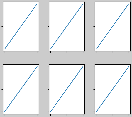
3 つ以上の列がある場合、wspaceはそれらの間で共有されるため、ここでは wspace を 2 つに分割し、各列の間のwspaceを 0.1 にします。

fig, axs = plt.subplots(2, 3, layout="constrained")
for ax in axs.flat:
    example_plot(ax, hide_labels=True)
fig.get_layout_engine().set(w_pad=4 / 72, h_pad=4 / 72, hspace=0.2,
                            wspace=0.2)

GridSpec にはオプションのhspaceおよびwspaceキーワード引数もあり、これらはによって設定されたパッドの代わりに使用されconstrained_layoutます。

fig, axs = plt.subplots(2, 2, layout="constrained",
                        gridspec_kw={'wspace': 0.3, 'hspace': 0.2})
for ax in axs.flat:
    example_plot(ax, hide_labels=True)
# this has no effect because the space set in the gridspec trumps the
# space set in constrained_layout.
fig.get_layout_engine().set(w_pad=4 / 72, h_pad=4 / 72, hspace=0.0,
                            wspace=0.0)

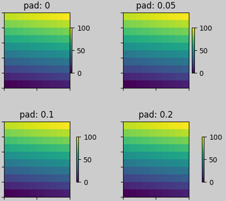
カラーバーによる間隔#

カラーバーは、親からパッドの距離に配置されます。ここで、パッド は、親の幅の一部です。次のサブプロットまでの間隔は、w/hspaceで指定されます。

fig, axs = plt.subplots(2, 2, layout="constrained")
pads = [0, 0.05, 0.1, 0.2]
for pad, ax in zip(pads, axs.flat):
    pc = ax.pcolormesh(arr, **pc_kwargs)
    fig.colorbar(pc, ax=ax, shrink=0.6, pad=pad)
    ax.set_xticklabels([])
    ax.set_yticklabels([])
    ax.set_title(f'pad: {pad}')
fig.get_layout_engine().set(w_pad=2 / 72, h_pad=2 / 72, hspace=0.2,
                            wspace=0.2)

rcParams #

スクリプトまたはファイルで設定できるrcParamsは 5 つありmatplotlibrc ます。それらにはすべて接頭辞がありますfigure.constrained_layout:

use : Constrained_layout を使用するかどうか。デフォルトは偽です
w_pad、h_pad : Axes オブジェクトの周りのパディング。インチを表す浮動小数点数。デフォルトは 3./72 です。インチ (3 ポイント)
wspace、hspace : サブプロットグループ間のスペース。分割されているサブプロット幅の割合を表す浮動小数点数。デフォルトは 0.02 です。

plt.rcParams['figure.constrained_layout.use'] = True
fig, axs = plt.subplots(2, 2, figsize=(3, 3))
for ax in axs.flat:
    example_plot(ax)

GridSpec で使用する#

Constrained_layout はsubplots()、、 subplot_mosaic()、または GridSpec()とともに使用することを意図していますadd_subplot()。

以下に注意してくださいlayout="constrained"

plt.rcParams['figure.constrained_layout.use'] = False
fig = plt.figure(layout="constrained")

gs1 = gridspec.GridSpec(2, 1, figure=fig)
ax1 = fig.add_subplot(gs1[0])
ax2 = fig.add_subplot(gs1[1])

example_plot(ax1)
example_plot(ax2)

より複雑な gridspec レイアウトが可能です。ここで、便利な関数add_gridspecとを使用していることに注意してくださいsubgridspec。

fig = plt.figure(layout="constrained")

gs0 = fig.add_gridspec(1, 2)

gs1 = gs0[0].subgridspec(2, 1)
ax1 = fig.add_subplot(gs1[0])
ax2 = fig.add_subplot(gs1[1])

example_plot(ax1)
example_plot(ax2)

gs2 = gs0[1].subgridspec(3, 1)

for ss in gs2:
    ax = fig.add_subplot(ss)
    example_plot(ax)
    ax.set_title("")
    ax.set_xlabel("")

ax.set_xlabel("x-label", fontsize=12)

Text(0.5, 41.33399999999999, 'x-label')

上の図では、左右の列の垂直範囲が同じではないことに注意してください。2 つのグリッドの上部と下部を並べたい場合は、同じグリッドスペックにある必要があります。軸が高さゼロにならないように、この図も大きくする必要があります。

fig = plt.figure(figsize=(4, 6), layout="constrained")

gs0 = fig.add_gridspec(6, 2)

ax1 = fig.add_subplot(gs0[:3, 0])
ax2 = fig.add_subplot(gs0[3:, 0])

example_plot(ax1)
example_plot(ax2)

ax = fig.add_subplot(gs0[0:2, 1])
example_plot(ax, hide_labels=True)
ax = fig.add_subplot(gs0[2:4, 1])
example_plot(ax, hide_labels=True)
ax = fig.add_subplot(gs0[4:, 1])
example_plot(ax, hide_labels=True)
fig.suptitle('Overlapping Gridspecs')

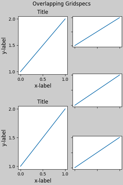
Text(0.5, 0.993055, 'Overlapping Gridspecs')

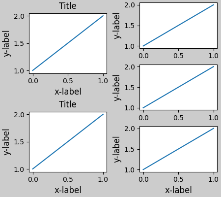
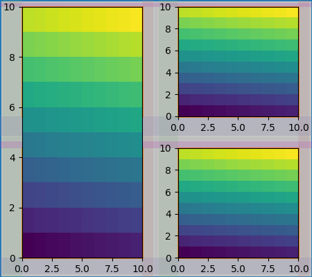
この例では、2 つの gridspec を使用して、カラーバーが 1 つの pcolor のセットのみに関連するようにします。このため、左側の列が右側の 2 つの列よりも幅が広いことに注意してください。もちろん、サブプロットを同じサイズにしたい場合は、必要なグリッドスペックは 1 つだけです。を使用しても同じ効果が得られることに注意してくださいsubfigures。

fig = plt.figure(layout="constrained")
gs0 = fig.add_gridspec(1, 2, figure=fig, width_ratios=[1, 2])
gs_left = gs0[0].subgridspec(2, 1)
gs_right = gs0[1].subgridspec(2, 2)

for gs in gs_left:
    ax = fig.add_subplot(gs)
    example_plot(ax)
axs = []
for gs in gs_right:
    ax = fig.add_subplot(gs)
    pcm = ax.pcolormesh(arr, **pc_kwargs)
    ax.set_xlabel('x-label')
    ax.set_ylabel('y-label')
    ax.set_title('title')
    axs += [ax]
fig.suptitle('Nested plots using subgridspec')
fig.colorbar(pcm, ax=axs)

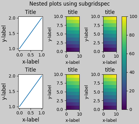
subgridspec、Title、Title、title、title、title、title を使用したネストされたプロット

<matplotlib.colorbar.Colorbar object at 0x7f2cdf471c30>

subgridspecs を使用する代わりに、Matplotlib は以下subfigures でも動作するものを提供するようになりましたconstrained_layout:

fig = plt.figure(layout="constrained")
sfigs = fig.subfigures(1, 2, width_ratios=[1, 2])

axs_left = sfigs[0].subplots(2, 1)
for ax in axs_left.flat:
    example_plot(ax)

axs_right = sfigs[1].subplots(2, 2)
for ax in axs_right.flat:
    pcm = ax.pcolormesh(arr, **pc_kwargs)
    ax.set_xlabel('x-label')
    ax.set_ylabel('y-label')
    ax.set_title('title')
fig.colorbar(pcm, ax=axs_right)
fig.suptitle('Nested plots using subfigures')

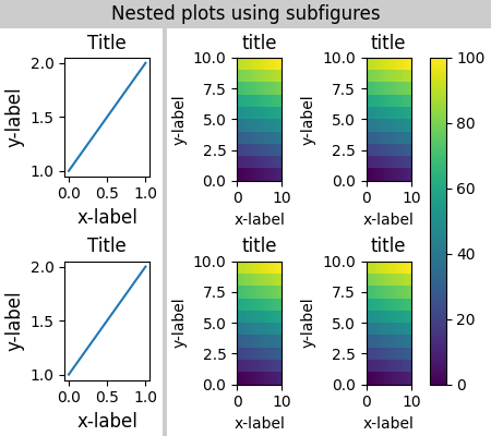
サブフィギュア、タイトル、タイトル、タイトル、タイトル、タイトル、タイトルを使用したネストされたプロット

Text(0.5, 0.9895825, 'Nested plots using subfigures')

軸位置の手動設定#

軸の位置を手動で設定する正当な理由がある場合があります。を手動で呼び出すとset_position、軸が設定されるため、constrained_layout はもう影響しません。constrained_layout(移動される軸のためのスペースが残っていることに注意してください)。

fig, axs = plt.subplots(1, 2, layout="constrained")
example_plot(axs[0], fontsize=12)
axs[1].set_position([0.2, 0.2, 0.4, 0.4])

固定縦横比軸のグリッド: 「圧縮」レイアウト#

constrained_layout軸の「元の」位置のグリッドで動作します。ただし、Axes の縦横比が固定の場合、通常は片側が短くなり、短くなった方向に大きな隙間ができます。以下では、Axes は正方形ですが、Figure は非常に幅が広いため、水平方向のギャップがあります。

fig, axs = plt.subplots(2, 2, figsize=(5, 3),
                        sharex=True, sharey=True, layout="constrained")
for ax in axs.flat:
    ax.imshow(arr)
fig.suptitle("fixed-aspect plots, layout='constrained'")

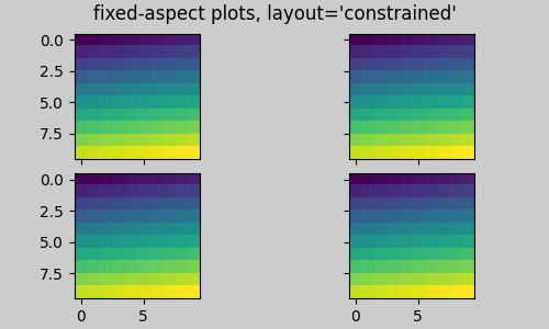
Text(0.5, 0.98611, "fixed-aspect plots, layout='constrained'")

これを修正する明白な方法の 1 つは、Figure のサイズをより正方形にすることですが、ギャップを正確に埋めるには試行錯誤が必要です。Axes の単純なグリッドの場合layout="compressed"、ジョブを実行するために使用できます。

fig, axs = plt.subplots(2, 2, figsize=(5, 3),
                        sharex=True, sharey=True, layout='compressed')
for ax in axs.flat:
    ax.imshow(arr)
fig.suptitle("fixed-aspect plots, layout='compressed'")

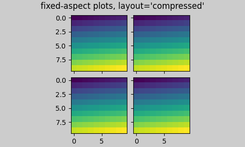
Text(0.5, 0.98611, "fixed-aspect plots, layout='compressed'")

手動でオフにする`constrained_layout`#

constrained_layout通常、図の描画ごとに軸の位置を調整します。によって提供される間隔を取得したいが constrained_layout、更新したくない場合は、最初の描画を行ってからを呼び出しますfig.set_layout_engine(None)。これは、目盛りラベルの長さが変わる可能性があるアニメーションに役立つ可能性があります。

ツールバーを使用するバックエンドの GUI イベントでconstrained_layoutはオフになっZOOMていることに注意してください。PANこれにより、ズームやパン中に軸の位置が変わるのを防ぎます。

制限事項#

互換性のない関数#

constrained_layoutはで動作しpyplot.subplotますが、各呼び出しで行と列の数が同じ場合のみです。その理由は、ジオメトリが同じでない場合、を呼び出すたびpyplot.subplotに新しいインスタンスが作成され、 . したがって、以下は正常に機能します。GridSpecconstrained_layout

fig = plt.figure(layout="constrained")

ax1 = plt.subplot(2, 2, 1)
ax2 = plt.subplot(2, 2, 3)
# third axes that spans both rows in second column:
ax3 = plt.subplot(2, 2, (2, 4))

example_plot(ax1)
example_plot(ax2)
example_plot(ax3)
plt.suptitle('Homogenous nrows, ncols')

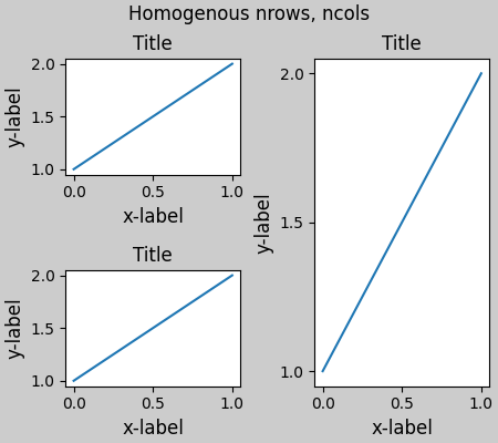
Text(0.5, 0.9895825, 'Homogenous nrows, ncols')

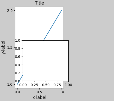
ただし、次の場合はレイアウトが不十分になります。

fig = plt.figure(layout="constrained")

ax1 = plt.subplot(2, 2, 1)
ax2 = plt.subplot(2, 2, 3)
ax3 = plt.subplot(1, 2, 2)

example_plot(ax1)
example_plot(ax2)
example_plot(ax3)
plt.suptitle('Mixed nrows, ncols')

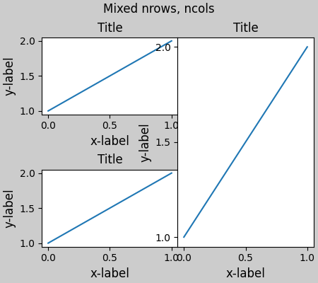
Text(0.5, 0.9895825, 'Mixed nrows, ncols')

同様に、 subplot2gridnrows と ncols はレイアウトの見栄えを良くするために変更できないという同じ制限で動作します。

fig = plt.figure(layout="constrained")

ax1 = plt.subplot2grid((3, 3), (0, 0))
ax2 = plt.subplot2grid((3, 3), (0, 1), colspan=2)
ax3 = plt.subplot2grid((3, 3), (1, 0), colspan=2, rowspan=2)
ax4 = plt.subplot2grid((3, 3), (1, 2), rowspan=2)

example_plot(ax1)
example_plot(ax2)
example_plot(ax3)
example_plot(ax4)
fig.suptitle('subplot2grid')

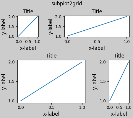
Text(0.5, 0.9895825, 'subplot2grid')

その他の注意事項#

constrained_layout目盛りラベル、軸ラベル、タイトル、および凡例のみを考慮します。したがって、他のアーティストがクリップされたり、オーバーラップしたりする場合があります。
目盛りラベル、軸ラベル、およびタイトルに必要な余分なスペースは、軸の元の位置とは無関係であると想定しています。多くの場合、これは当てはまりますが、そうでない場合がまれにあります。
バックエンドがレンダリングフォントを処理する方法にはわずかな違いがあるため、結果はピクセル単位で一致しません。
Axes の境界を超えて拡張された Axes 座標を使用するアーティストは、Axes に追加されると異常なレイアウトになります。Figureこれは、アーティストを using に直接追加することで回避できます add_artist()。例については、を参照 ConnectionPatchしてください。

デバッグ#

Constrained-layout は、予期しない方法で失敗する可能性があります。制約ソルバーを使用するため、ソルバーは数学的に正しいソリューションを見つけることができますが、ユーザーが望んでいるものとはまったく異なります。通常の失敗モードは、すべてのサイズが最小許容値に崩壊することです。これが発生した場合は、次の 2 つの理由のいずれかが原因です。

描画をリクエストしていた要素のための十分なスペースがありませんでした。
バグがあります - その場合は https://github.com/matplotlib/matplotlib/issuesで問題を開きます。

バグがある場合は、外部データや依存関係 (numpy 以外) を必要としない自己完結型の例を報告してください。

アルゴリズムに関する注意事項#

制約のアルゴリズムは比較的単純ですが、図をレイアウトする方法が複雑なため、多少複雑になります。

Matplotlib でのレイアウトは、クラスを介して gridspecs で実行されGridSpecます。gridspec は、Figure を行と列に論理的に分割したもので、これらの行と列の Axes の相対的な幅はwidth_ratiosとheight_ratiosで設定されます。

Constrained_layout では、各 gridspec はそれに関連付けられたlayoutgridを取得します。layoutgridは、列ごとに一連の and 変数、行ごとに一連のleftand変数を持ち、さらに左、右、下、上にそれぞれマージンを持ちます。各行で、その行のすべてのデコレーターが収まるまで、上下のマージンが広げられます。列と左右の余白についても同様です。rightbottomtop

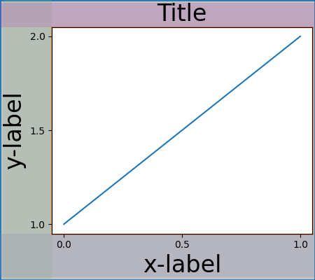
単純なケース: 1 つの軸#

単一の軸の場合、レイアウトは簡単です。1 つの列と行で構成される Figure の 1 つの親 layoutgrid と、1 つの行と列で構成される軸を含む gridspec の子 layoutgrid があります。軸の両側に「装飾」用のスペースが作られています。コードでは、これは次のdo_constrained_layout()ようなエントリによって実現されます。

gridspec._layoutgrid[0, 0].edit_margin_min('left',
      -bbox.x0 + pos.x0 + w_pad)

bbox軸のタイトなバウンディングボックスとposその位置はどこにありますか。4 つの余白が軸の装飾をどのように取り囲んでいるかに注目してください。

from matplotlib._layoutgrid import plot_children

fig, ax = plt.subplots(layout="constrained")
example_plot(ax, fontsize=24)
plot_children(fig)

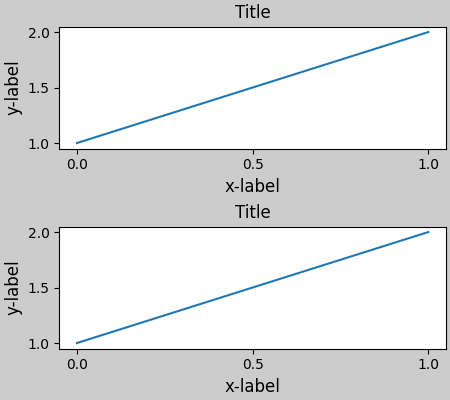
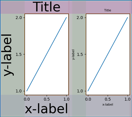
単純なケース: 2 つの軸#

複数の軸がある場合、それらのレイアウトは簡単な方法でバインドされます。この例では、左の軸は右の軸よりもはるかに大きな装飾を持っていますが、大きな xlabel を収容するのに十分な大きさの下部余白を共有しています。共有上マージンと同じです。左マージンと右マージンは共有されないため、異なっていてもかまいません。

fig, ax = plt.subplots(1, 2, layout="constrained")
example_plot(ax[0], fontsize=32)
example_plot(ax[1], fontsize=8)
plot_children(fig)

2 つの軸とカラーバー#

カラーバーは、親のレイアウトグリッドセルのマージンを拡張する単なる別のアイテムです。

fig, ax = plt.subplots(1, 2, layout="constrained")
im = ax[0].pcolormesh(arr, **pc_kwargs)
fig.colorbar(im, ax=ax[0], shrink=0.6)
im = ax[1].pcolormesh(arr, **pc_kwargs)
plot_children(fig)

Gridspec に関連付けられたカラーバー#

カラーバーがグリッドの複数のセルに属する場合、それぞれのマージンが大きくなります。

fig, axs = plt.subplots(2, 2, layout="constrained")
for ax in axs.flat:
    im = ax.pcolormesh(arr, **pc_kwargs)
fig.colorbar(im, ax=axs, shrink=0.6)
plot_children(fig)

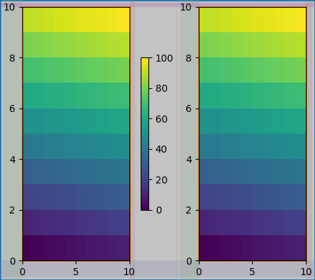
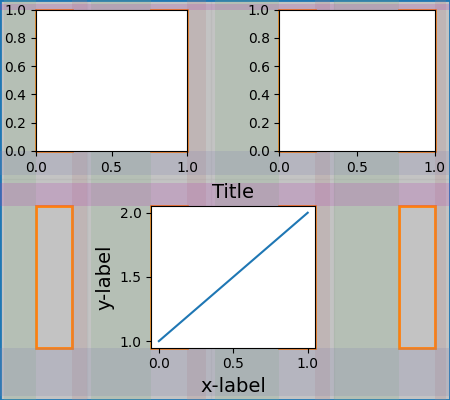
不均一なサイズの軸#

Gridspec レイアウトで軸のサイズを不均一にするには、Gridspec の行または列を横切るように指定する方法と、幅と高さの比率を指定する方法の 2 つがあります。

ここでは最初の方法を使用します。中央topと bottom余白は左側の列の影響を受けないことに注意してください。これはアルゴリズムの意識的な決定であり、右側の 2 つの軸が同じ高さを持つケースにつながりますが、左側の軸の高さの 1/2 ではありません。gridspecこれは、制約されたレイアウトなしで機能する方法と一致しています。

fig = plt.figure(layout="constrained")
gs = gridspec.GridSpec(2, 2, figure=fig)
ax = fig.add_subplot(gs[:, 0])
im = ax.pcolormesh(arr, **pc_kwargs)
ax = fig.add_subplot(gs[0, 1])
im = ax.pcolormesh(arr, **pc_kwargs)
ax = fig.add_subplot(gs[1, 1])
im = ax.pcolormesh(arr, **pc_kwargs)
plot_children(fig)

微調整が必要なケースの 1 つは、余白の幅を制限するアーティストがいない場合です。以下の例では、列 0 の右マージンと列 3 の左マージンには幅を設定するマージンアーティストがいないため、アーティストがいるマージン幅の最大幅を使用します。これにより、すべての軸が同じサイズになります。

fig = plt.figure(layout="constrained")
gs = fig.add_gridspec(2, 4)
ax00 = fig.add_subplot(gs[0, 0:2])
ax01 = fig.add_subplot(gs[0, 2:])
ax10 = fig.add_subplot(gs[1, 1:3])
example_plot(ax10, fontsize=14)
plot_children(fig)
plt.show()

スクリプトの合計実行時間: ( 0 分 18.885 秒)

Sphinx-Gallery によって生成されたギャラリー

制約付きレイアウト ガイド#

簡単な例#

カラーバー#

副題番号

伝説#

パディングとスペース#

カラーバーによる間隔#

rcParams #

GridSpec で使用する#

軸位置の手動設定#

固定縦横比軸のグリッド: 「圧縮」レイアウト#

手動でオフにするconstrained_layout#

制限事項#

互換性のない関数#

その他の注意事項#

デバッグ#

アルゴリズムに関する注意事項#

単純なケース: 1 つの軸#

単純なケース: 2 つの軸#

2 つの軸とカラーバー#

Gridspec に関連付けられたカラーバー#

不均一なサイズの軸#

制約付きレイアウトガイド#

手動でオフにする`constrained_layout`#